Excel line chart with target range
You can also go through our other suggested articles Checklist in Excel. Change the color by changing the Colors on the Page Layout tab.
3 Ways To Add A Target Line To An Excel Pivot Chart
Chartwithtargetrangezip 14kb 30-Oct-13 CH0007 - Show Sparklines for Hidden Data -- Macro changes all sparklines on the active sheet so they will show data even if rows and columns are hidden.
. In this column a simple formula using the MAX function returns the largest value in your data range. Achievement chart but target line method is simple effective. Step 2 Insert the Doughnut Chart.
In my example I added 50 but if you are working with larger. The Chart Type dialog box opens. Another way is.
I set the Y axis scale as follows. With the data range set up we can now insert the doughnut chart from the Insert tab on the Ribbon. Now select the colored charts that correspond to Min the top-most layer Max and Result and make the following conversions.
A vertical line appears in your Excel bar chart and you just need to add a few finishing touches to make it look right. Under the Axis label range select the axis values from the original data. If none of the predefined combo charts.
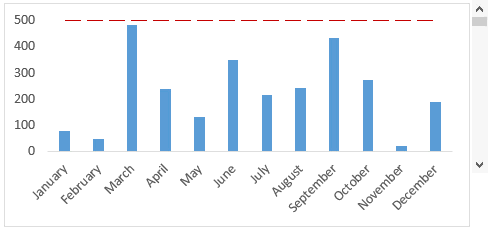
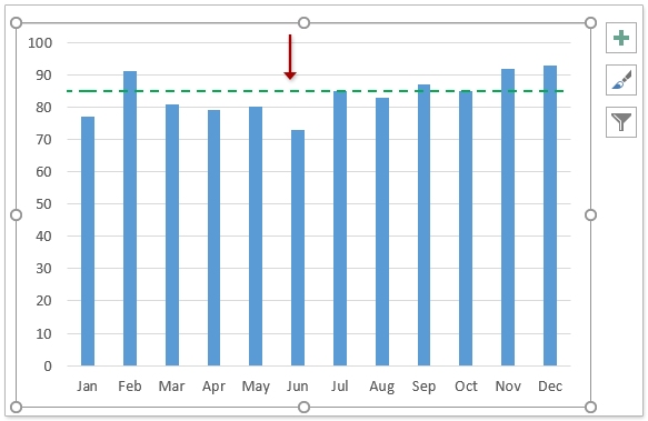
If the target value series is the second series in the chart in this step you need to right click at the Target Value series. CH0008 - Show Target Range on Line Chart -- Show sales quantity in a line chart with target range shown in the background. Chart types line scatter and ribbon even cone same happens when I change the number.
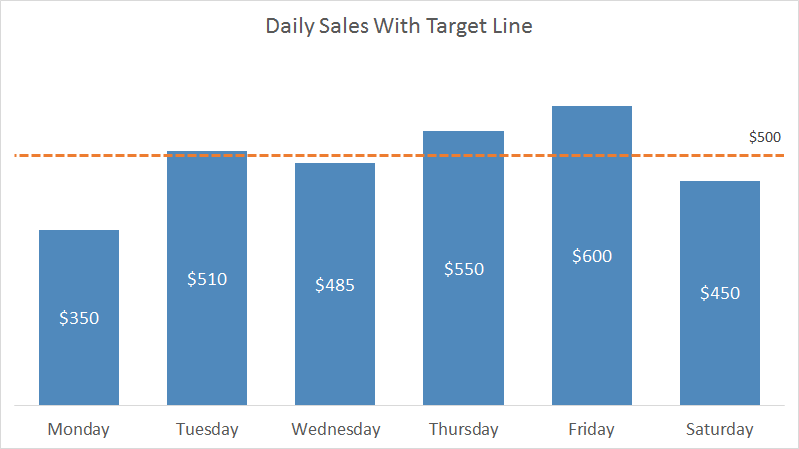
Instead of a formula enter your target values in the last column and insert the Clustered Column - Line combo chart as shown in this example. In the inserted chart right click at the Actual Value seriesthen in the context menu click Format Data Series. Excel 2007 2010.
Now from the table select all the values from the min row. The same technique can be used to plot a median For this use the MEDIAN function instead of AVERAGE. Now go to the Combo option and check the Secondary Axis box for the Percentage of Students Enrolled columnThis will add the secondary axis in the original chart and will separate the two charts.
Select in the Design tab. Surface Charts in Excel. The entire chart will be shaded with the progress complete color and we can display the progress percentage in the label to show that it is greater than 100.
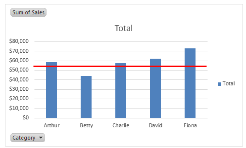
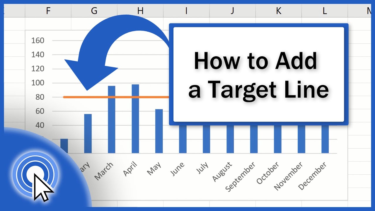
Add a Horizontal Target Line in Column Chart. A common task is to add a horizontal line to an Excel chart. Then click Ctrl C to copyNow click on the chart and hit Ctrl V to pasteThis will result in an additional layer being added to the stacked chart as shown below.
If you will try to apply formatting from one chart for example bar chart to some other type of chart for example line chart it will also change the type of target chart. There are several other ways to create a Target Vs. I change the charted data range to 160 or more rows of data 155 to all 1050 and suddenly the labels become random.
Double-click the secondary vertical axis or right-click it and choose Format Axis from the context menu. When you add data labels to a chart series excel can show either category series or data point values as data labels. From the Design tab choosethe Chart Style.
Now you dont have to worry about formatting multiple charts. I hope you found this tip. 2In the popped out Progress Bar Chart dialog box please do the following operations.
Add a cushion to the formula so that none of your target lines are at the very top of the chart. 3D Scatter Plot in Excel. Click Kutools Charts Progress Progress Bar Chart see screenshot.
You have a super quick method to copy chart formatting to another excel chart. Min 8 PM 083333 Max 10 AM 1416667 and Major Unit 2 hours 008333. Displaying graph elements Data Labels Gridlines Graph Title.
Adding a target line or benchmark line in your graph is even simpler. In the Format Axis pane under Axis Options type 1 in the Maximum bound box so that out vertical line extends all the way to the top. Target values as bars.
Select Chart Styles and Layout on the Design tab. Excel 2013 2016 2019 365. After inserting the chart two contextual tabs will appearnamely Design and Format.
Select Percentage of current completion option if you want to create the progress bar chart. Select the range of data go to the insert tab click on column chart click on 2D chart. This is used to cover the vertical lines of the target bars in the column chart.
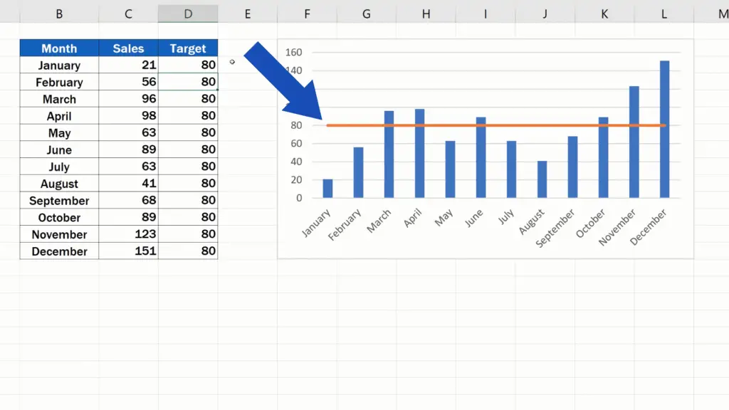
This is one more method which I often use in my charts is adding a target line. First of all let me show you the data which I am using to create a target line in the chart. Select the data range and click Insert Insert Column or Bar Chart Clustered ColumnSee screenshot.
To the left of the top chart copy the range select the chart and use Paste Special to add the data to the. The Doughnut Chart is in the Pie Chart drop-down. Click the brush icon on the top right of the graph to select Chart Styles and Colors.
Radar Chart in Excel. The horizontal line may reference some target value or limit and adding the horizontal line makes it easy to see where values are above and below this reference value. Here we discuss how to create excel animation chart along with practical examples and a downloadable excel template.
This is a guide to Excel Animation Chart. To add the reference line in the chart you need to return the average of sales amount. After installing Kutools for Excel please do as this.
Select the Chart - Right Click on it - Change Chart Type. Plot in a line chart. You can make it even more interesting if you select one of the line series then select UpDown Bars from the Plus icon next to the chart in Excel 2013 or the Chart Tools Layout tab in 20072010.
These features are in. Select the Chart - Design - Change Chart Type.

Line Chart Line Chart Actual With Forecast Exceljet
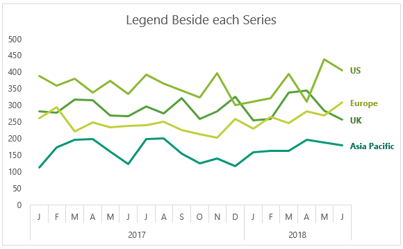
Dynamically Label Excel Chart Series Lines My Online Training Hub
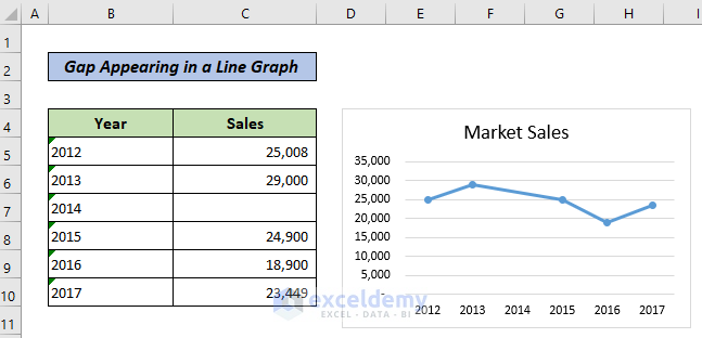
Line Graph In Excel Not Working 3 Examples With Solutions
Create Dynamic Target Line In Excel Bar Chart
Combo Chart Column Chart With Target Line Exceljet
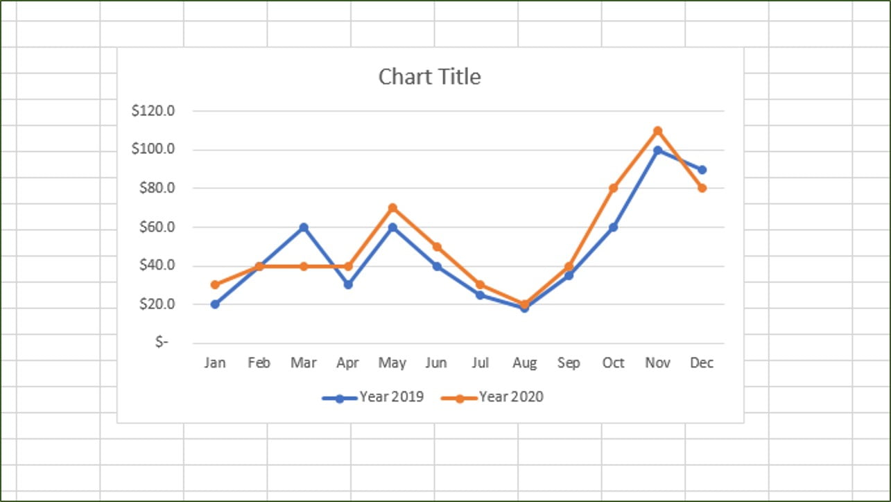
How To Make A Line Graph In Excel With Multiple Lines
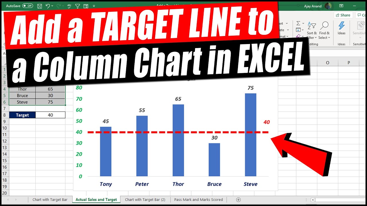
How To Add A Target Line To A Column Chart 2 Methods Youtube
How To Add Horizontal Benchmark Target Base Line In An Excel Chart

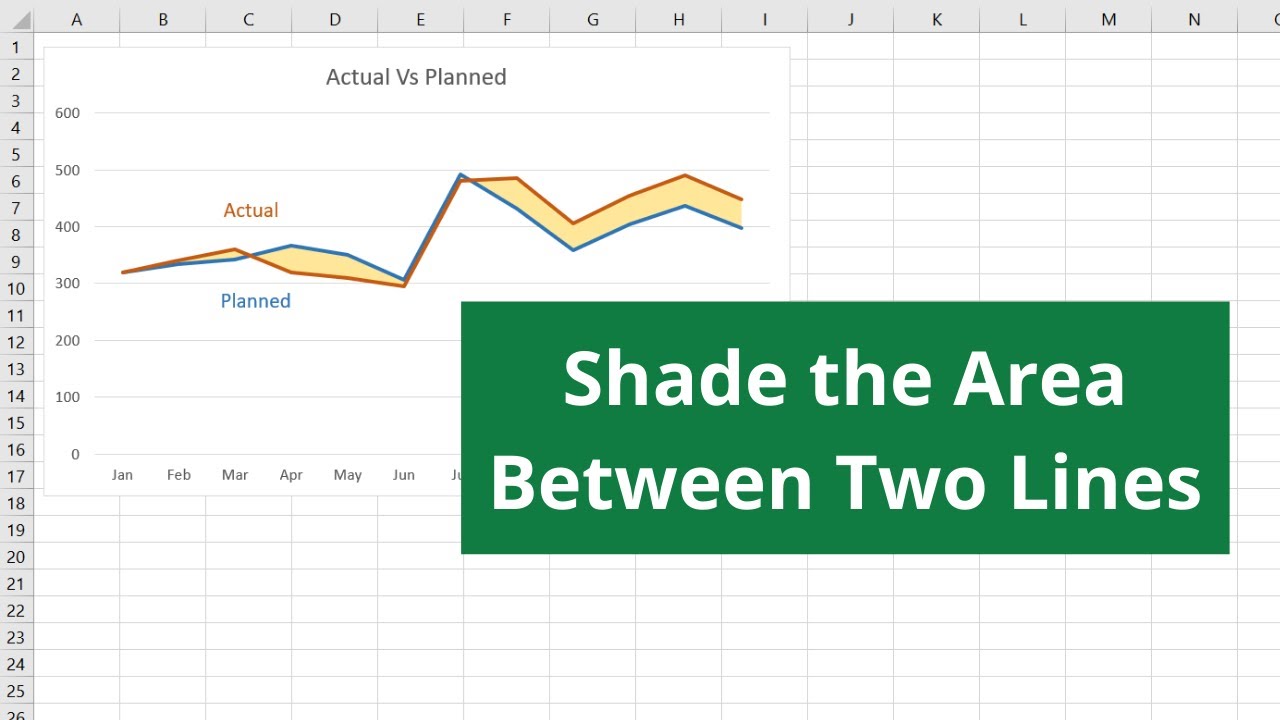
Excel Variance Charts Making Awesome Actual Vs Target Or Budget Graphs How To Pakaccountants Com Excel Excel Shortcuts Excel Tutorials
Line Graph With A Target Range In Excel Youtube
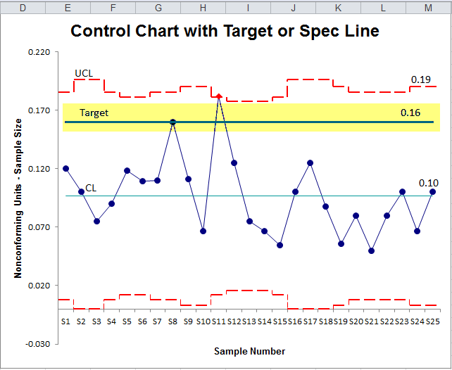
Add Target Line Or Spec Limits To A Control Chart

How To Add Horizontal Benchmark Target Base Line In An Excel Chart

Data Visualization Chart 75 Advanced Charts In Excel With Video Tutorial Data Visualization Data Visualization Infographic Chart Infographic
How To Add A Target Line In An Excel Graph
How To Add A Target Line In An Excel Graph Youtube

Bullet Charts Vertical And Horizontal From Visual Graphs Pack Graphing Chart Data Visualization
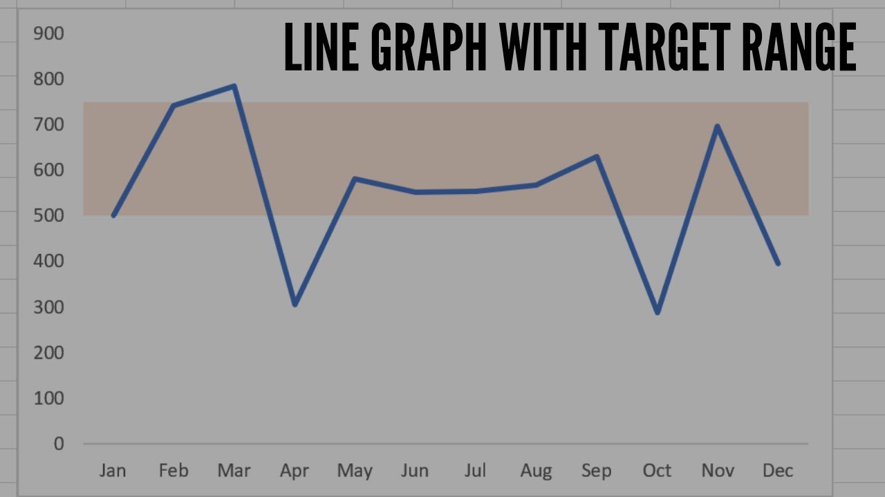
Line Graph With A Target Range In Excel Youtube